
I've taken over running dbplanview.com.
If you spend any time with a database, you'll eventually find some queries which are inexplicably slow.
The first step to making those queries faster is to know what the database was thinking: this is as easy as running the query with explain in front of it. Or adding explain analyze before the query, to show both the plan and the how long each stage actualy took.
But the output is complicated — a lot happens in parallel — which is why some sort of visualization is needed. dbplanview.com, creates this visualization.
In this query, we get source_id from route, and use this in a query on source:
travelinedata=> select * from source where source_id = (select source_id from route where description = 'Fen Street - Agora');
If we run the query with explain or explain analyze at the start:
travelinedata=> explain select * from source where source_id = (select source_id from route where description = 'Fen Street - Agora');
The database will output:
                                   QUERY PLAN
---------------------------------------------------------------------------------
 Index Scan using source_pkey on source  (cost=3089.34..3097.35 rows=1 width=36)
   Index Cond: (source_id = $0)
   InitPlan 1 (returns $0)
     ->  Seq Scan on route  (cost=0.00..3089.05 rows=6 width=4)
           Filter: (description = 'Fen Street - Agora'::text)
(5 rows)
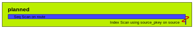
Copy-paste into dbplanview.com and click "Timeline", and this timeline will be displayed, with time running from left-to-right:
Querying route uses a sequential scan, which takes lots of time (it checks each row). Querying source uses an index and takes less time.
The joining line means the output of "seq scan on route" is used in the "index scan on source". It's red because the index scan doesn't start until the first stage has finished.
The example above is equaivalent to this join:
travelinedata=> explain select * from route join source using (source_id) where route.description = 'Fen Street - Agora';
Which the database plans like this:
                                   QUERY PLAN
---------------------------------------------------------------------------------
 Nested Loop  (cost=0.29..3138.93 rows=6 width=36)
   ->  Seq Scan on route  (cost=0.00..3089.05 rows=6 width=4)
         Filter: (description = 'Fen Street - Agora'::text)
   ->  Index Scan using source_pkey on source  (cost=0.29..8.30 rows=1 width=36)
         Index Cond: (source_id = route.source_id)
(5 rows)
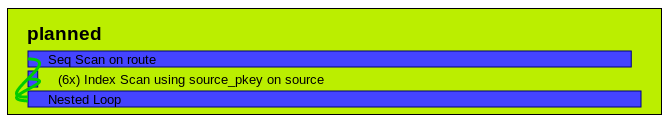
The output of "seq scan on route" is still used in the "index scan on source", but the index scan doesn't wait. It runs in parallel: as soon as route gets a result, an index scan will be performed.
The index scan probably won't happen immediately (as the diagram sort-of suggests), it happens whenever the sequential scan gives a result. The query planner expects there to be 6 results from "seq scan on route" (so the index scan will probably happen 6 times).
The "nested loop" takes the output of both index and sequential scan and sticks them together. It appears to take a long time, but it's not really the slow bit: it spends most of its time waiting for the other parts of the query to finish.
If you do have slow queries:
Try and rephrase the query to make better use of indexes. \d+ tablename shows the indexes availble. You might wish to add an index, but this will make inserts and updates to that table more costly: think carefully about the ratio of update vs select before adding any index.
The planner treats with as a barrier: the query inside the with will fully complete before the next query starts. For example, select * from route limit 10 will stop reading route once it has 10 rows. But with foo as (select * from route) select * from foo limit 10 will read all of route into memory (as "foo"), then take the first 10.
Cache expensive queries using a materialized view.
Adjust the query planner costs to favour a different approach. One common way is to set local random_page_cost to 0; to make indexes infinitely more favourable than an sequential scan (for the transaction).
That's all there is to it! Give dbplanview.com a go, to work out where your queries are slow.